My name is Derek Fan. I am a
student, engineer, developer, and learner.

I implemented the A* search algorithm to be used as an offline path planner for UAV Forge's autonomous drone, a senior design project that participates in the AUVSI SUAS competition. The main requirements for the offline planner were for it to generate a path that would pass through waypoints and avoid pre-defined obstacles in the shortest amount of time.

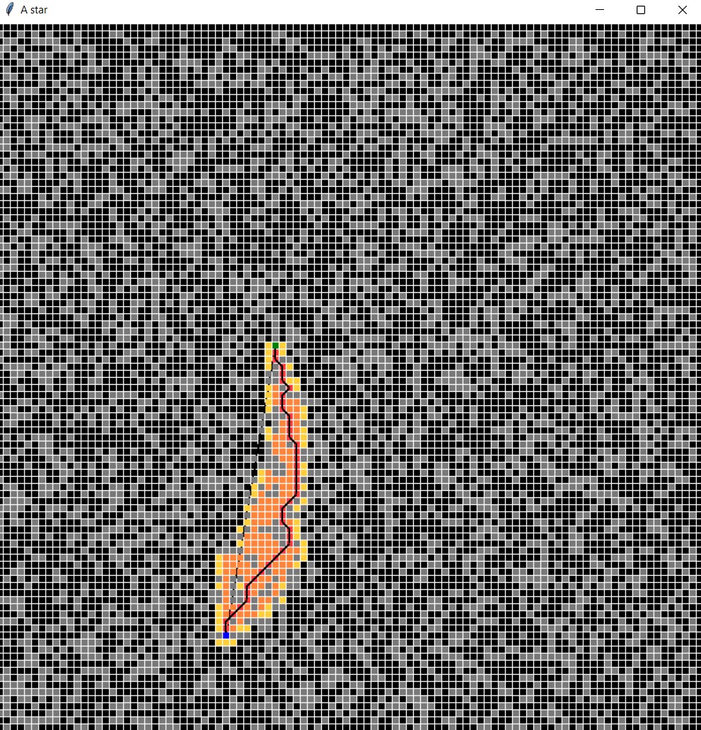
Above is an example of the algorithm successfully finding the shortest path from a start to goal node through an obstacle-filled environment. The gray tiles or nodes represent randomly generated obstacles that cannot be traveled through.

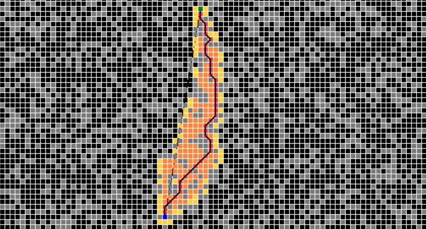
Here is a clearer view of the figure. The blue and green nodes are the start and goal, respectively. The yellow nodes represent spaces the algorithm has "seen" but not actually traveled to. The orange nodes are alternate paths that the algorithm has explored. Finally, the red is the final path that yields the least distance.

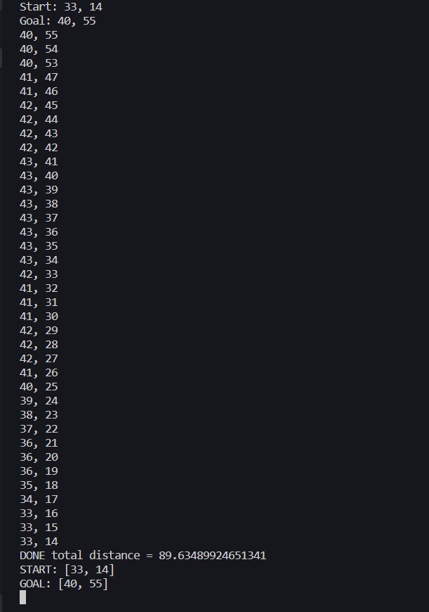
Above is a representation of the path as a series of x-y coordinates. So how exactly does this algorithm work?

A* is essentially a "guided" version of Djikstra's algorithm, which seeks to map out every node in the environment of interest before deciding on the shortest path available. Djikstra's follows the cost function f(n) = g(n), which states that the cost f at every node is a value g that represents the difficulty to reach node n. The shortest path will minimize this cost function. However, before it can calculate the ideal route, Djikstra's must assign costs to every possible node. While exploring nodes, it exhibits a behavior akin to trickling water branching in every available direction. In an open environment with g-costs associated with distance, this is not computationally feasible.

A* builds upon the idea of minimizing a cost function by revising it to f(n) = g(n) + h(n). This new term is the heuristic cost, an estimate of the difficulty of reaching the goal from node n. In most scenarios, this is simply the distance between the current node and goal. The cost at every node is therefore its distance from the start in addition to its distance from the end. The closer a node is to the goal, the smaller its cost will be. The addition of the heuristic directs the Djikstra's random "trickle" into streams that will always progress towards the goal. This is apparent in the first image, where the colored tiles largely highlighted a path towards the end node.

Although A* will almost always return an optimal path, it is not without its weaknesses. For one, it has a large space complexity attributed to the need to store all explored nodes before calculating the shortest path. It is slower to compute than the likes of RRT (rapidly-exploring random tree), and demands certainty and information in its environemnt to be successful in real-world scenarios.